ROMS-IMLE: A Minimalist Approach to Competitive Single-Step Generative Modelling

Which parts of modern generative modelling actually matter? Starting from IMLE and adding back only the essentials: we achieve FID 2.56 on ImageNet 256 in a single step.

Abstract

Generative models have undergone many generations of evolution, from VAEs/GANs to diffusion/flow matching. Along the way, the underlying techniques have become more complicated and various beliefs about what drives strong empirical performance have taken hold. Due to the success of diffusion models and flow matching, one of the more common beliefs is the importance of transforming the noise distribution to the data distribution gradually through many small transformations.

We ask whether this is truly necessary, and take a minimalist approach to designing a competitive generative model. We start with the bare-bones essentials, namely just a training objective and a model. We purposefully make both simple. For the training objective, we choose Implicit Maximum Likelihood Estimation (IMLE), and eschew more complicated alternatives such as variational inference, adversarial training and numerical integration. For the model, we eschew transformers and instead choose a moderately sized convolutional network. Then we judiciously added elements that are truly essential, which surprisingly do not include iterative denoising. The result is a single-step parameter-efficient generative model that produces high quality samples at fast speed: it achieves an FID of 2.56 on ImageNet 256 and simultaneously attains good precision and recall.

Background

Flow Matching and Diffusion Models

Stochastic interpolant models, which includes diffusion and flow matching models, currently define the state of the art in image generation. They succeeded earlier approaches such as GANs, which are unstable to train and prone to mode collapse, and VAEs, which train stably but tend to produce blurry, low-fidelity samples.

Their advantage is commonly attributed to how they decompose generation. Instead of mapping the prior distribution to the data distribution in one large transformation, they break the mapping into a sequence of smaller, simpler transformations. Each of these transformations is typically carried out by a separate step in the sampling process, and as a result sampling takes many steps to iterate over all the transformations.

Generating in a Single Step with IMLE

Implicit Maximum Likelihood Estimation takes a direct route: a neural generator maps samples from the prior to data samples in a single pass.

IMLE is a single step model: IMLE model can directly produce accurate samples in one single step.

Training such a generator directly is generally difficult because the likelihood of the data under it is intractable. IMLE provides a workaround, implicitly maximizing that likelihood without requiring it to be known explicitly. IMLE optimizes a likelihood-based objective akin to regression, without the variational bounds and encoders of VAEs, the adversarial training of GANs, or the iterative numerical integration used by stochastic interpolant models.

Formally, IMLE learns a direct mapping \(f_\theta\) from a prior \(\pi(\mathbf{z})\) to the data distribution \(p_\mathrm{data}(\mathbf{x})\) by minimizing

\[\theta_{\text{IMLE}} = \arg\min_\theta \; \mathbb{E}_{\mathbf{z}_1, \ldots, \mathbf{z}_m \sim \pi(\mathbf{z})} \left[ \sum_{i=1}^{n} \min_{j \in [m]} \; d\left( \mathbf{x}_i, f_\theta(\mathbf{z}_j) \right) \right],\]

where \(d(\cdot, \cdot)\) is a distance.

To optimize the objective, the IMLE algorithm alternates between two phases. In the matching phase, $m$ latent codes \(\mathbf{z}_1, \ldots, \mathbf{z}_m\) are sampled from the prior and each real image \(\mathbf{x}_i\) is matched to its nearest generated sample in the set \(\{f_\theta(\mathbf{z}_1), \ldots, f_\theta(\mathbf{z}_m)\}\). This establishes a coupling between \(\pi(\mathbf{z})\) and \(p_\mathrm{data}(\mathbf{x})\). Next, in the optimization phase, the parameters \(\theta\) are updated to bring each generated sample closer to its matched real image.

Overview of IMLE algorithm: First, each real data point is coupled with its nearest generated sample. Next, the model's parameters are updated to reduce the distance within each coupled pair.

Can Minimalism Be Competitive?

This paper asks a simple question: is all of the machinery that modern generative models have accumulated, from elaborate architectures to sophisticated sampling schemes and intricate training objectives, truly necessary? Rather than add to it, we take a minimalist approach: we start from the simplest generative model we can, IMLE, and add only the components that prove essential. In line with the same minimalist philosophy, we use a ConvNeXt-based architecture rather than the transformer-based ones that now dominate. We identify one improvement to each of IMLE’s two phases.

Improvements to IMLE

Optimization Phase: Supervising Every Stage

An Alternative View of Diffusion/Flow Matching Models

Stochastic interpolant methods are commonly understood to perform iterative denoising. At test time, that network is applied repeatedly to convert pure noise into a generated sample. Consider an alternative view of these models under a deterministic sampler (like DDIM or Flow Matching models). Rather than viewing the model as one instance of the denoising network, we unroll the iterations of the sampler and view the model as their composition, \(h_\theta = g^1_\theta \circ \cdots \circ g^T_\theta\), where \(g^t_\theta\) is the update applied at iteration \(t\). This allows us to view the reverse process as a single compositional model \(h_{\theta}\), that maps a sample from the prior \(\mathbf{x}_T\) to a data sample \(\mathbf{x}_0\). Under this view, each \(\mathbf{x}_{t-1} = g^t_{\theta}(\mathbf{x}_t)\) is an intermediate layer of \(h_{\theta}\).

Read this way, the training objective reveals something specific. SI methods supervise the denoising network’s prediction at every time step, with equal weight applied to all steps, so every intermediate layer of \(h_\theta\) receives a direct training signal. We call this per-stage supervision, and we hypothesize that the sample quality of many-step models stems from it rather than from iterative sampling itself.

Compositional view of reverse process: The reverse process can be viewed as a single compositional model, and the training objective supervises every layer of this model directly. We hypothesize that this per-stage supervision, and not iterative sampling, is what drives sample quality.

Adapting Multi-Stage Supervision for IMLE

The IMLE generator can also be seen as a prior-to-data network composed of stages, only executed in a single forward pass rather than through iterative sampling. We build it as a stack of upsampling blocks, \(f_\theta = f_{\theta^{L}} \circ \cdots \circ f_{\theta^{1}}\), in which each stage operates at a progressively higher resolution. This recasts IMLE in a form similar to the diffusion construction, with each stage \(f_{\theta}^{l}\) now analogous to \(g^t_\theta\), only indexed by resolution rather than noise level.

In existing IMLE methods, the loss is computed only at the final output, which directly supervises only the last stage. We address this by supervising every stage directly, at the resolution at which it operates. Concretely, we add a per-stage output head so that each stage outputs an image at its own resolution, and obtain its target by downsampling the real image.

Optimization phase improvement: Vanilla IMLE only supervises the final resolution. We change this so that each stage is directly supervised through downsampled targets.

Matching Phase: Making Matching Robust

Outliers from Randomness in Sampling

For the IMLE algorithm, the model distribution changes during training, so the matching between model samples and ground truth data points needs to be recomputed. Due to randomness in the sampling, there may be no samples drawn from a mode of the model distribution, and as a result, a ground truth data point that can otherwise be explained by that mode would not be well matched. Note that this is different from mode collapse: the poor matching results from randomness in the sampling, not a deficiency in the model distribution.

Randomness in Sampling: Matching is recomputed every round from a fresh set of samples, so an unlucky draw can leave a real data point with no sample near it. This is a sampling artefact rather than mode collapse.

A Robust Loss

The standard squared $l_2$ loss lets these mismatches dominate the mean loss. In essence this is a problem of outliers: a small number of large-residual mismatched pairs contribute disproportionately to the mean loss compared to a much larger pool of well-matched pairs.

The classical remedy in robust statistics is to replace the squared $l_2$ loss with a function that grows sub-quadratically in the residual, so that a mismatch has less influence and the well-matched pairs dominate the update. Empirically, we find that Geman-McClure loss works best in our case.

Matching phase improvement: Replacing squared $l_2$ loss with a robust loss like Geman-McClure loss makes the matching phase robust to outliers caused by randomness in sampling.

Putting It All Together

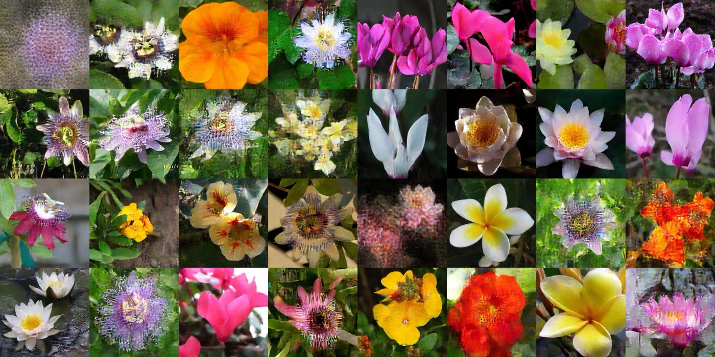
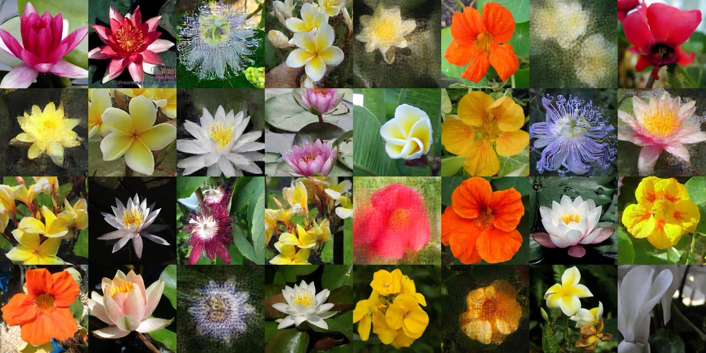
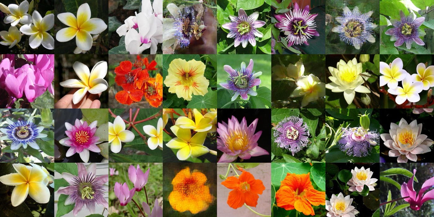
We call the resulting method ROMS-IMLE, short for Robust Multi-Stage Implicit Maximum Likelihood Estimation. We ablate our contributions on Oxford Flowers dataset (1000 images $256 \times 256$).

Configuration	FID ↓	Precision ↑	Recall ↑
Vanilla IMLE	62.61 ± 2.28	0.45 ± 0.03	0.46 ± 0.01
IMLE + Multi-Stage	31.24 ± 1.08	0.79 ± 0.01	0.72 ± 0.02
IMLE + Multi-Stage + Geman-McClure (ours)	13.90 ± 0.08	0.93 ± 0.00	0.73 ± 0.02

Ablation on Oxford Flowers: We report the mean and standard deviation over three seeds, all evaluated at the same training iteration.

Vanilla IMLE: FID 62.61

IMLE + Multi-Stage: FID 31.24

IMLE + Multi-Stage + Geman-McClure: FID 13.90

Results

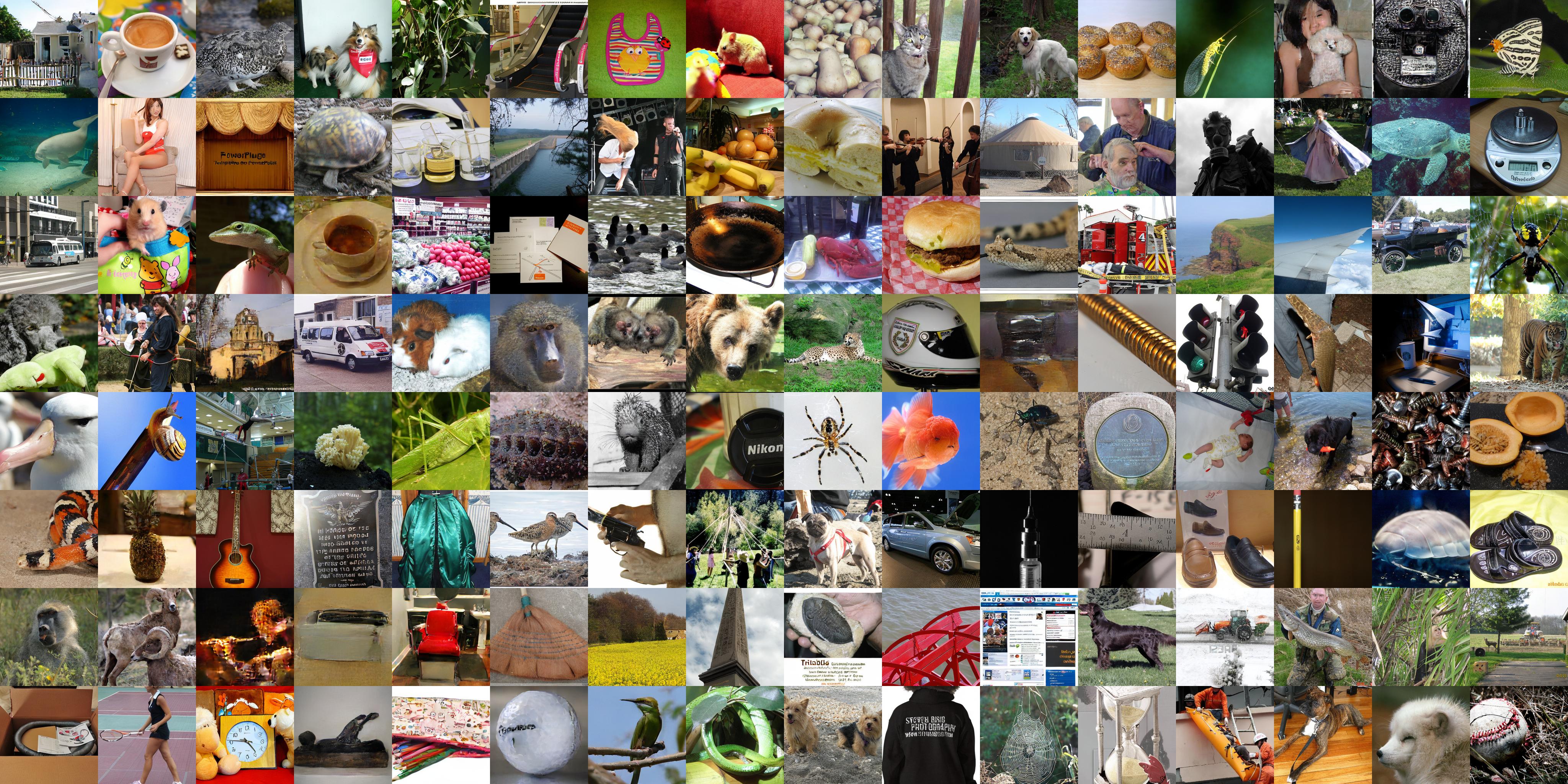
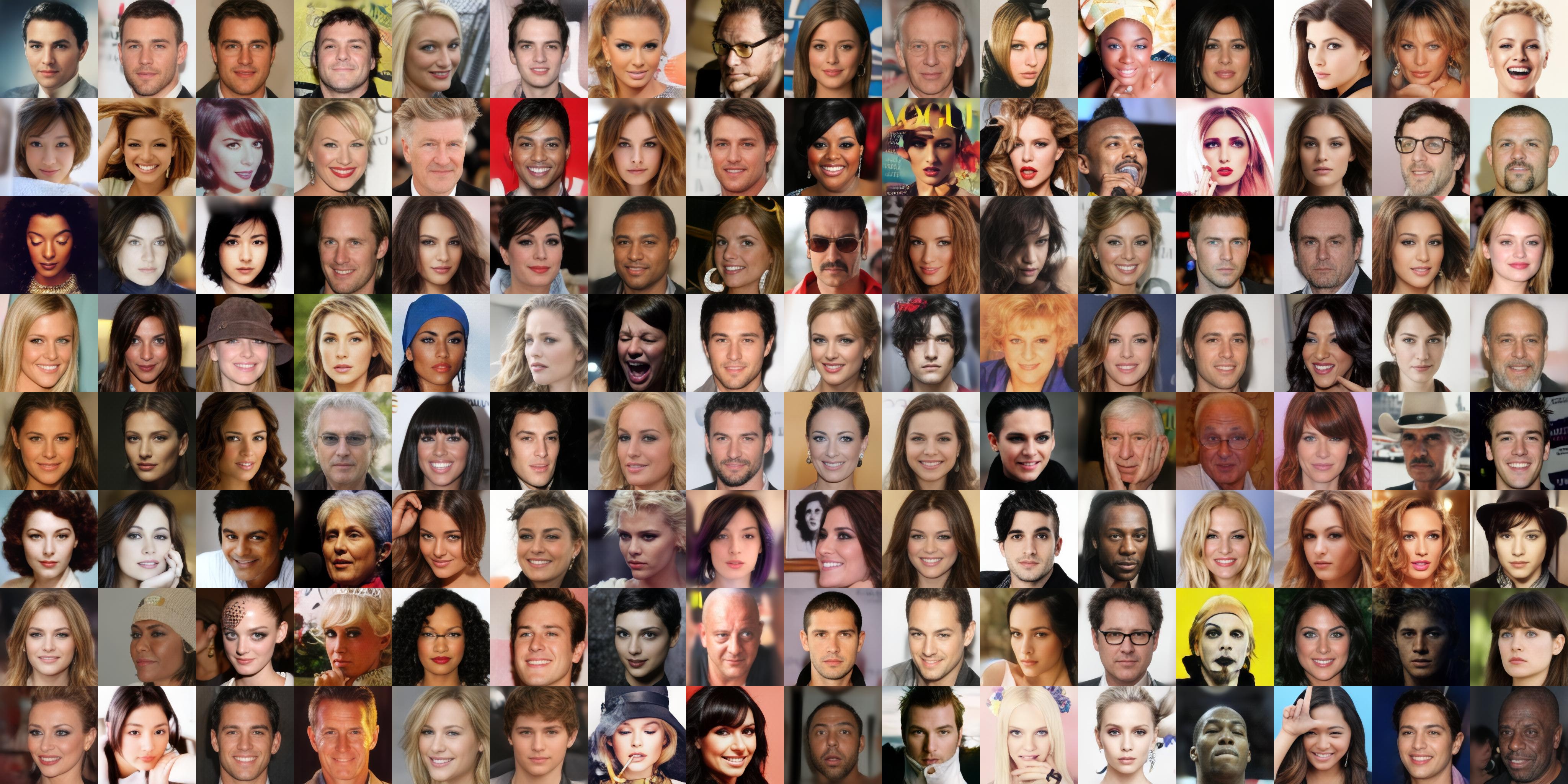
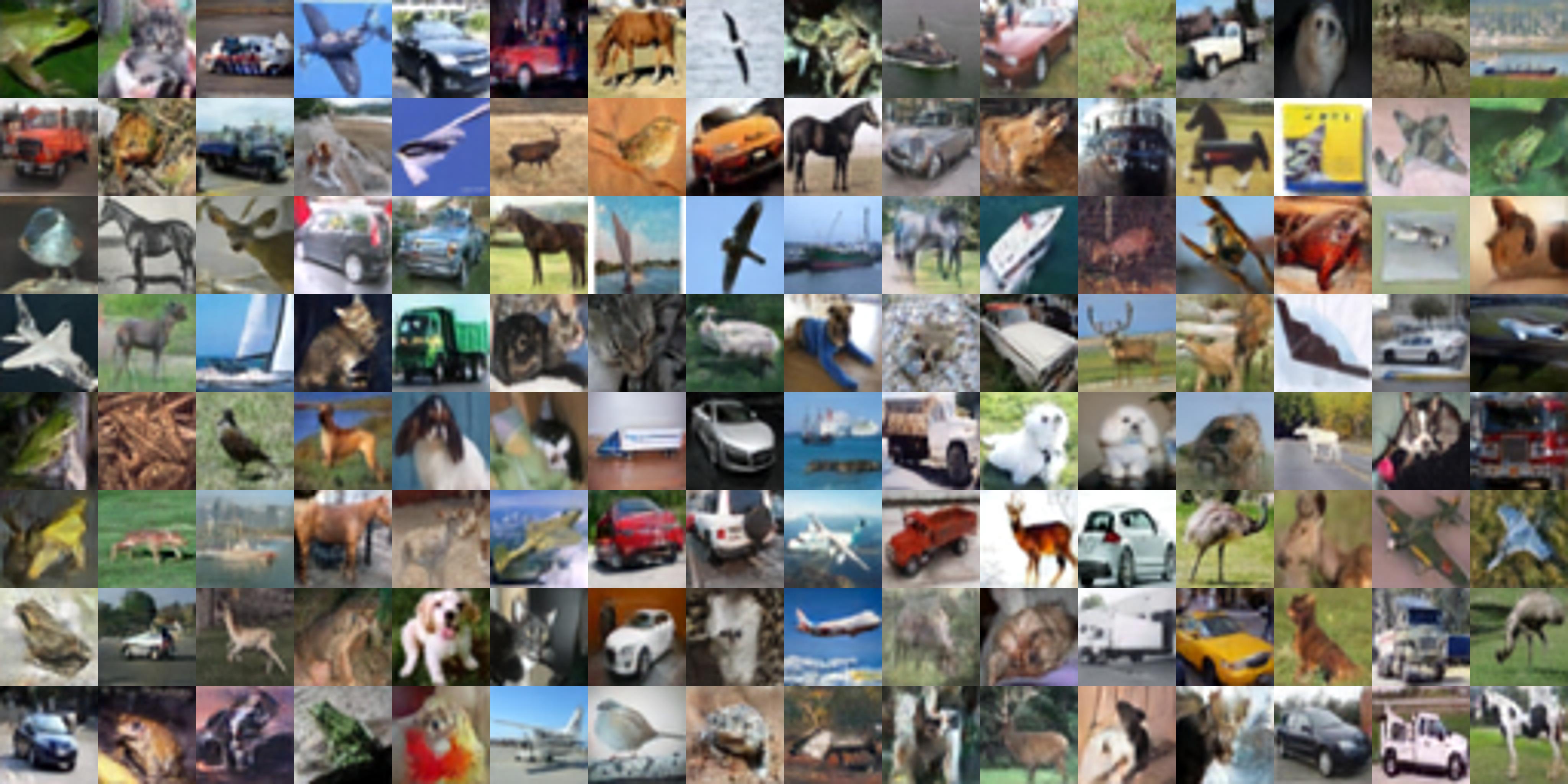
Our approach works well in both pixel and latent space.

ImageNet 256 [Latent]: FID 2.56, 310M params, 1 NFE

CelebA-HQ [Pixel]: FID 6.70, 138M params, 1 NFE

CIFAR-10 [Pixel]: FID 3.93, 1 NFE

Interpolating in prior space: Each tile in the 7 × 4 grid is a separate interpolation. Moving linearly between two prior samples produces plausible images that vary smoothly, suggesting the generator has learned a coherent mapping from the prior.

BibTeX

@article{vashist2026romsimle,
  title={ROMS-IMLE: A Minimalist Approach to Competitive Single-Step Generative Modelling},
  author={Vashist, Chirag and Li, Ke},
  journal={arXiv preprint arXiv:2607.19332},
  year={2026}
}